Stock Prediction with PyCaret
PyCaret is an open-source, low-code machine learning library in Python that automates machine learning workflows. It is an end-to-end machine learning and model management tool that speeds up the experiment cycle exponentially and makes you more productive.
Introduction
Recently PyCaret announced their new Time Series module. In this article, we build a stock predictor Python application using PyCaret.
Acquiring Stock Prices
Yahoo Finance has a Python library that can be used to fetch stock data based on the stock ticker. Yahoo Finance library can be added using
pip install yfinancethen to fetch all available data on let say Apple Inc [AAPL], we run the following code

we need only the close price so, we discard other columns, by using
data = data[[‘Close’]]
also, we need to reset the index, as currently the date column is taken as the index.

Convert TimeSeries to Frequency
Next, we use pandas dataframe.asfreq function to convert the time series data to daily frequency(d). We also use the pandas ffill function to replace any null values with nearest values.
We also need to make the date column in DateTime format, to ensure this we first convert it to string and then use pd.to_datetime function.

Generating Prediction Model
We use pyCaret to generate the prediction model. It can be installed using
pip install pycaret-ts-alphaInitializing the setup
We initialize using the setup function to which we pass the dataset and strategy
from pycaret.time_series import *
setup(data, fh = 7, fold = 3, session_id = 123)
Compare and select the best model
This will train and select the best model after evaluating all of them
best = compare_models()
Prediction
Once the model is generated, we can use the predict_model function to generate predicted data passing the model and duration. This output is as Pandas Series, so we use to_frame function to convert it to a data frame.
prediction = predict_model(best, fh = 90)
prediction.to_frame()
prediction
Aggregate and Visualise
We need to reset the index and again convert to frequency. The timestamp of prediction is in periods. We can now add both the historic and predicted data. Let us also add 50 and 200-day moving averages.
complete = data.append(prediction)
complete.reset_index(level=0, inplace=True)
complete.columns = ['Date','Close']
complete = addfreq(complete)
complete['MA50']=complete['Close'].rolling(50).mean()
complete['MA200']=complete['Close'].rolling(200).mean()
complete
We use Plotly Express, to create the graph
complete = complete_data(data, prediction)
fig = px.line(complete)
fig.show()

Summary
A final program would be as follows